Useful documents for engineering students of CSE, and specially for students of aryabhatta knowledge university, Bihar (A.K.U. Bihar). It covers following topics: Disk structure, disk scheduling (FCFS, SSTF, SCAN, C-SCAN)

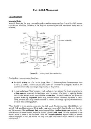
1. Unit IX: Disk Management
Disk structure
Magnetic Disks
Magnetic Disks are the most commonly used secondary storage medium. It provides high storage
capacity and reliability. Following is the diagram representing the disk mechanism along with its
structure.
Details of the components are listed here:
● Each disk platter has a flat circular shape, like a CD. Common platter diameters range from
1.8 to 5.25 inches. The two surfaces of a platter are covered with a magnetic material. We
store information by recording it magnetically on the platters.
● A read-write head "flies" just above each surface of every platter. The heads are attached to
a disk arm that moves all the heads as a unit. The surface of a platter is logically divided
into circular tracks, which are subdivided into sectors. The set of tracks that are at one arm
position makes up a cylinder. There may be thousands of concentric cylinders in a disk
drive, and each track may contain hundreds of sectors. The storage capacity of common disk
drives is measured in gigabytes.
When the disk is in use, a drive motor spins it at high speed. Most drives rotate 60 to 200 times per
second. Disk speed has two parts. The transfer rate is the rate at which data flow between the drive
and the computer. The positioning time, sometimes called the random-access time, consists of the
time necessary to move the disk arm to the desired cylinder (seek time). The time necessary for the
desired sector to rotate to the disk head, called the rotational latency. Typical disks can transfer
several megabytes of data per second, and they have seek times and rotational latencies of several
milliseconds.

2. Because the disk head flies on an extremely thin cushion of air (measured in microns), there is a
danger that the head will make contact with the disk surface. Although the disk platters are coated
with a thin protective layer, the head will sometimes damage the magnetic surface. This accident is
called a head crash. A head crash normally cannot be repaired; the entire disk must be replaced.
A disk can be removable, allowing different disks to be mounted as needed. Removable magnetic
disks generally consist of one platter, held in a plastic case to prevent damage while not in the disk
drive. Floppy disks are inexpensive removable magnetic disks that have typically storage capacity
of only 1.44MB or so. While removable disks are available that work much like normal hard disks
and have capacities measured in gigabytes. The head of a floppy-disk drive generally sits directly
on the disk surface, so the drive is designed to rotate more slowly than a hard-disk drive to reduce
the wear on the disk surface.
Magnetic Tapes
Magnetic Tapes was used as an early secondary-storage medium. Although it is relatively
permanent and can hold large quantities of data, its access time is slow compared with that of main
memory and magnetic disk. In addition, random access to magnetic tape is about a thousand times
slower than random access to magnetic disk, so tapes are not very useful for secondary storage.
Tapes are used mainly for backup, for storage of infrequently used information, and as a medium
for transferring information from one system to another.
A tape is kept in a spool and is wound or rewound past a read-write head. Moving to the correct
spot on a tape can take minutes, but once positioned, tape drives can write data at speeds
comparable to disk drives. Tape capacities vary greatly, depending on the particular kind of tape
drive. Typically, they store from 20GB to 200GB. Some have built-in compression that can more
than double the effective storage. Tapes and their drivers are usually categorized by width, including
4, 8 and 19 millimeters and 1/4 and 1/2 inch.
Disk scheduling
One of the responsibilities of the operating system is to use the hardware efficiently. For the disk
drives, meeting this responsibility includes having fast access time and large disk bandwidth. The
access time has two major components:
• Seek Time: It is the time for the disk arm to move the heads to the cylinder containing the
desired sector.
• Rotational Latency: It is the additional time for the disk to rotate the desired sector to the
disk head.
The disk Bandwidth is the total number of bytes transferred, divided by the total time between the
first request for service and the completion of the last transfer. We can improve both the access time
and the bandwidth by managing the order in which disk I/O requests are serviced.
Whenever a process needs I/0 to or from the disk, it issues a system call to the operating system.
The request specifies several pieces of information:
• Whether this operation is input or output
• What is the disk address for the transfer
• What is the memory address for the transfer
• What is the number of sectors to be transferred
If the desired disk drive and controller are available, the request can be serviced immediately. If the
drive or controller is busy, any new requests for service will be placed in the queue of pending

3. requests for that drive. For a multiprogramming system with many processes, the disk queue may
often have several pending requests. Thus, when one request is completed, the operating system
chooses which pending request to service next. The operating system make this choice based on one
of several disk-scheduling algorithms, which are discussed below:
FCFS scheduling
The simplest form of disk scheduling is, of course, the first-come, first-served (FCFS) algorithm.
This algorithm is intrinsically fair, but it generally does not provide the fastest service. Consider, for
example, a disk queue with requests for I/0 to blocks on cylinders:
98, 183, 37, 122, 14, 124, 65, 67
If the disk head is initially at cylinder 53, it will first move from 53 to 98, then to 183, 37, 122, 14,
124, 65, and finally to 67, for a total head movement of 640 cylinders.
SSTF Scheduling
It seems reasonable to service all the requests close to the current head position before moving the
head far away to service other requests. This assumption is the basis for the Shortest-Seek-Time-
First (SSTF) algorithm. The SSTF algorithm selects the request with the least seek time from the
current head position. Since seek time increases with the number of cylinders traversed by the head,
SSTF chooses the pending request closest to the current head position.
For our example request queue, the closest request to the initial head position (53) is at cylinder 65.
Once we are at cylinder 65, the next closest request is at cylinder 67. From there, the request at
cylinder 37 is closer than the one at 98, so 37 is served next. Continuing, we service the request at
cylinder 14, then 98, 122, 124, and finally 183 (as shown in following figure).

4. This scheduling method results in a total head movement of only 236 cylinders-little more than one
third of the distance needed for FCFS scheduling of this request queue. Clearly, this algorithm gives
a substantial improvement in performance.
SSTF scheduling is essentially a form of shortest-job-first (SJF) scheduling; and like SJF
scheduling, it may cause starvation of some requests. Remember that requests may arrive at any
time. Suppose that we have two requests in the queue, for cylinders 14 and 186, and while the
request from 14 is being serviced, a new request near 14 arrives. This new request will be serviced
next, making the request at 186 wait. While this request is being serviced, another request close to
14 could arrive. In theory, a continual stream of requests near one another could cause the request
for cylinder 186 to wait indefinitely.
Although the SSTF algorithm is a substantial improvement over the FCFS algorithm, it is not
optimal. In the example, we can do better by moving the head from 53 to 37, even though the latter
is not closest, and then to 14, before turning around to service 65, 67, 98, 122, 124, and 183. This
strategy reduces the total head movement to 208 cylinders.
SCAN Scheduling
In the SCAN algorithm , the disk arm starts at one end of the disk and moves toward the other end,
servicing requests as it reaches each cylinder, until it gets to the other end of the disk. At the other
end, the direction of head movement is reversed, and servicing continues. The head continuously
scans back and forth across the disk. The SCAN algorithm is sometimes called the elevator
algorithm, since the disk arm behaves just like an elevator in a building, first servicing all the
requests going up and then reversing to service requests the other way.
Before applying SCAN to schedule the requests on cylinders 98, 183,37, 122, 14, 124, 65, and 67
(as per our example), we need to know the direction of head movement in addition to the head's
current position. Assuming that the disk arm is moving toward 0 and that the initial head position is
again 53, the head will next service 37 and then 14. At cylinder 0, the arm will reverse and will
move toward the other end of the disk, servicing the requests at 65, 67, 98, 122, 124, and 183 (given
in figure below).
Quiz 1: What is the total head movement (SCAN scheduling)?
If a request arrives in the queue just in front of the head, it will be serviced almost immediately; a
request arriving just behind the head will have to wait until the arm moves to the end of the disk,
reverses direction, and comes back.

5. C-SCAN Scheduling
Circular SCAN (C-SCAN) is a variant of SCAN designed to provide a more uniform wait time.
Like SCAN, C-SCAN moves the head from one end of the disk to the other, servicing requests
along the way. When the head reaches the other end, however, it immediately returns to the
beginning of the disk without servicing any requests on the return trip (see the figure below).
Quiz2: What is the total head movement (C-SCAN scheduling)?
The C-SCAN scheduling algorithm essentially treats the cylinders as a circular list that wraps
around from the final cylinder to the first one.
LOOK and C-LOOK scheduling
As SCAN and C-SCAN, both move the disk arm across the full width of the disk In practice,
neither algorithm is often implemented this way. More commonly, the arm goes only as far as the
final request in each direction. Then, it reverses direction immediately, without going all the way to
the end of the disk. Versions of SCAN and C-SCAN that follow this pattern are called LOOK and
C-LOOK scheduling because they look for a request before continuing to move in a given
direction. The head movement for C-LOOK scheduling is shown in following figure for the same
example, which differs from the traces of C-SCAN scheduling at end-points.

6. Given so many disk-scheduling algorithms, how do we choose the best one?
SSTF is common and has a natural appeal because it increases performance over FCFS. SCAN and
C-SCAN perform better for systems that place a heavy load on the disk, because they are less likely
to cause a starvation problem.
With any scheduling algoritlunf however, performance depends heavily on the number and types of
requests. For instance, suppose that the queue usually has just one outstanding request. Then, all
scheduling algorithms behave the same because they have only one choice of where to move the
disk head: they all behave like FCFS scheduling.
Previous Years Questions:
1. Explain the working of LOOK and C-LOOK scheduling algorithms. (8)
(Year 2013, aku)
2. (a) What do you understand by disk scheduling? Describe seek time and rotational latency.
(6)
(b) describe SCAN scheduling. How is C-SCAN different from SCAN? (8)
(Year 2013, aku)
3. (a) Is disk scheduling other than FCFS scheduling useful in a single-user environment?
Explain your answer.
(b) Suppose that a disk drive has 5000 cylinders, numbered 0 to 4999. The drive is currently
serving a request at cylinder 143 and the previous request was at cylinder 125. The queue of
pending requests in FIFO order is 86, 1470, 913, 1774, 948, 1509, 1022, 1750, 130. Stsrting
from the current head position, what is the total distance (in cylinders) that the disk arm
moves to satisfy all the pending requests for each of the following disk-scheduling
algorithms?
I. SSTF
II. SCAN
III. C-SCAN (7)
(Year 2015, aku)
Important Questions:
1. Compare the functionalities of FCFS, SSTF, C-SCAN and C-LOOK disk scheduling
algorithms with an example for each.
2. Given the following queue 95, 180, 34, 11, 123, 62, 64 with head initially at track 50 and
ending at track 199. Calculate the number of moves using FCFS, SSTF, Elevator and C-
LOOK algorithm. Also show the graphical representation.
3. What is disk scheduling? Explain any 3 disk scheduling methods with examples.