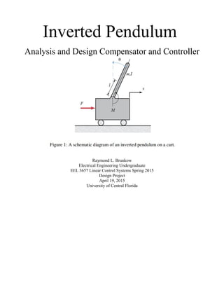
1. Inverted Pendulum
Analysis and Design Compensator and Controller
Raymond L. Brunkow
Electrical Engineering Undergraduate
EEL 3657 Linear Control Systems Spring 2015
Design Project
April 19, 2015
University of Central Florida

2. Abstract:
This paper develops the design and implementation of optimized algorithm for motion control of an
inverted pendulum and cart system. The real time access of position of the pendulum is the feedback to
the controller and pre-compensator. The process is visually represented via the use of Matlab.
Through Matlab you are able to see both the uncompensated and the compensated system in action.
Modeling and Position Control of an Inverted Pendulum on a Cart.
An inverted pendulum is mounted on a cart as shown in Figure 1. The cart is capable of moving in the
horizontal direction on rails once “bumped” with an impulse force, F. The pendulum is hinged to the
cart at the bottom of its length such that it moves in the same plane as the cart. With no pendulum
angle controller implemented, the mounted inverted pendulum is free to fall along the horizontal axis.
The applied force is provided to the cart by a servo-mechanism that involves a dc motor, a pulley, and a
belt. The inverted pendulum system is to be controlled to maintain upright position for the pendulum
when the cart moves and to reject disturbance. The block diagram of the inverted pendulum
compensated system is displayed in Figure 2. The position feedback sensor has a transfer gain of 2.864
V/rad/sec. The transfer function of the servo-mechanism actuator is given by:
Km R(M +m) s
τm s+1
System parameters and their values to be used for simulation are tabulated in Table 1.

3. System Modeling and Simulation
For the Inverted Pendulum system, consider applied force, F as system input and pendulum
angle, ϴ as system output:
1) Determine the dynamic equations of motion for the system (Nonlinear system model)
2) Build a Simulink model to represent the Inverted Pendulum dynamic equations of
motion and obtain system transfer function, TF1.
3) Analytically linearize the dynamic equations of motion to obtain system transfer
function, TF2. Assume small change in the pendulum angle is around the upright
position.
4) Use Matlab/Simulink to compare the uncompensated unit step output response of the
aforementioned three representations of the inverted pendulum system.
Pendulum Angle Controller Design
Design a PID controller or a phase lead/lag compensator using root locus methods to satisfy the
following design requirements for a unit step and impulse inputs:
Settling time of less then 0.5 seconds.
No steady state error.
Overshoot of less then 20%
Test your compensated system
Mathematics:

4. Using the two free body diagrams above the summation of forces in the horizontal direction is:
[1] M ¨x+b ˙x+N=F
Ignoring the summation of forces in the vertical direction as that is not a direction of movement for this
design program. The force exerted on the pendulum in the horizontal direction is:
[2] N=m ¨x+m I ¨Θcos(Θ)−m I ˙Θ
2
sin(Θ)
Substitution and solving for both the F and Angular equations we have the following:
[3] (M +m) ¨x+b ˙x+m I ¨Θcos(Θ)−m I ˙Θ2
sin(Θ)=F
[4] (I +m I
2
) ¨Θ+mgIsin(Θ)=mI ¨x cos(Θ)
These two equations provide us with the non-linear equations or the dynamic equations of motion for
the inverted pendulum system.
Building this into a Simulink model we have the following block diagram:

5. With the following functions for Xddot, Thetaddot, N, P, Theta:
¨x=
1
M
(F−N −b ˙x)
¨Θ=
1
I
(−NlCos(Θ)−Plsin(Θ))
N =m( ¨x−l ˙Θ
2
sin (Θ)+l ¨Θcos(Θ))
P=m(l ˙Θcos(Θ)l ¨Θsin(Θ+g))
Θ=
1
π
Setting Theta to 1 over π indicates the starting position of vertical. This can be combined into a much
simpler subsystem:
Linearlizing the dynamic equations [3] and [4] we make a few assumptions:
1) Θ = π + Φ, such that Φ is the small angle around the vertical stable position.

6. 2)
cos(Θ)=−1
sin(Θ)=−Φ
d Θ2
dt
=0
Taking the Laplace transforms of [3] and [4] we have the following:
(M +m) ¨x+b ˙x−m I ¨Φ=u
(I +mI
2
) ¨Φ−mgI Φ=mI ¨x
Solving the system of equations of Angular position over Output we have the following TF1:
Φ(s)
U (s)
=
ml⋅s
α⋅s+b( I+mI
2
)⋅s
2
−mgI (M +m)⋅s−bmgI
α=(M +m)( I+mI
2
)−(mI)
2
Neglecting friction from the design specification in Table 1 we are left with the linearized transfer
function for the inverted pendulum system in the time domain:
Φ(s)
U ( s)
=
K p
s
2
Ap
2
−1
K p=
1
(M +m) g
Ap=±
√(
(M +m)mgI
(M +m)(I +mI2
)−(mI )2
)
Φ(t)
u(t)
=
K p
D
2
Ap
2
−1
Pulley, Belt, Cart, and Motor
The load-inertia to the motor consists of a pulley with a radius of R and the mass of the card plus the
mass of the pendulum. Torque provided to the motor is shown below:
T L=(M +m)⋅r
2
⋅D ω
To calculate the dynamics of the motor the following set of equations are used such that τ is the time
constant and depends on the load drive.
ω=Km
E
τ D+1
U (s)
E(s)
=Km
(M +m)rs
( τm s+1)
The overall transforms function TF2 for the combined system uncompensated open loop is:
Φ(s)
E(s)
=K
s
(τm s+1)(
s
2
Ap
2
−1)
K=K F KP K M r(M +m)
E(s)=ErrorVoltage
Φ(s)=Angular position of the pendulum

7. Forward path transfer function:
Closed-Loop transfer function for the inverted pendulum:

8. Analysis of Uncompensated System:
Pole Zero open loop uncompensated system:
Impulse response open loop uncompensated system:

9. Step response open loop uncompensated system:
Root locus uncompensated system:

10. From the root locus of the uncompensated system it is clear to see that there is a pole in the right half
plane, thus the system currently is unstable. This is the crux of the project to create a PID controller
that will maintain stability under unit step and impulse inputs. After the creation of the PID controller a
new root locus will be displayed that will maintain the design specification.
Compensator Design:
Using the root locus method combined with the sisotool, mathematics, and some guidance from the
professor the following gains for the PID plus a cascading controller were generated:
The compensator equation is found to be:
Gc=K c (
KD⋅s
2
+K P⋅s+KI
s
)
KC =8, KP=20, K I =100, K D=1
This provided fair results, but by adding the cascading controller with a value of 30 the following are
the gain results: KC =30 KP=20 K I=100 K D=1
Analysis of the Compensated System:
Currently the block diagram matches the design specification with the Gc in series with the servo-
mechanism and the inverted pendulum all providing the position feedback to the summation point as
depicted in Figure 2.
The PID controller provides a pole at the origin to negate the original zero from the plant, plus two
zeros at -10 to pull the root locus away from the imaginary access and further into the left half plane for
stability.

11. In order the root locus to remain stable the gain K > 0.8. By doing so all of the root locus will reside in
the left half plane and thus be stable.
Impulse response closed loop compensated system:
Step response closed loop controlled system:

12. Note that the DC state never reaches the goal of zero steady state error. The error is roughly 65%. Far
to great. To eliminate the steady state error an Integral controller needs to be added to the system as a
pre-compensator. Below is the results:
With roughly 8% overshoot and a settling time of 0.194 seconds the design is well within the
specification of this project.
Transfer function for PID controller:
Closed-Loop transfer function for controlled
system:

13. DC Gain for closed-loop controlled system is 0.3502, upon adding the pre-compensator to the system
the transfer function becomes:
Conclusion:
Throughout the design process the driving factor has been to master the tools of the trade, specifically
Matlab. While the transfer functions and much of the math is found on the internet, the manipulation
of those functions and diagrams are meaningless unless you are able to utilize Matlab or some other
graphical tool to represent all of the available data points and potential options without spending hours
or even days guessing and testing new values for the controllers.
While I was able to generate numerical values for KC, KP, KI, KD, having the KC = 30 as a scalar
provides a KI = 3000. This is unrealistic from a potential cost point of view. This controlled system
would work amazing in real life if money was not an object to prevent its manufacturing. The speed
that the system returns to stability to the human eye would be virtually instant at less then 2 10th
of a
second.
Matlab code:
%------------------------------------------------------------------------
% data
% Design project EEL 3657 Linear Controls Spring 2015
% By Raymond L. Brunkow
% Data for the Inverted Pendulum on movable cart
%------------------------------------------------------------------------
%%%% Data provided as part of design project
M = 0.9; % mass of cart in Kg
m = 0.1; % mass of pendulum in Kg
l = 0.235; % Length of pendulum to Center of Gravity m

14. I = 0.0053; % Moment of Inertia of Pendulum Kg m^2
r = 0.023; % radius of pully m
tau_m = 0.5; % time constant of motor s
Km =17; % gain of motor rad/s/V
Kf = 2.864; % feedback gain V/rad/s
b = 0; % friction of cart
g = 9.8; % gravity m/s
% Force applied to the cart by the pulley mechanism = u
% Cart Position = x
% Pendulum Angle off the vertical = theta
%----------------------------------------------------------------------------
% Open Loop & Closed Loop (Uncontroled) Transfer Function
%----------------------------------------------------------------------------
%
% E U
% Position --->O--->[ G2 ]--->[ G1 ]---+---> Theta
% - ^ |
% | | Theta = sys * E
% +----------[ H ]<----------+
%
Kp = 1 / ((M + m) * g); % 1
% Kp = --------
% g(M + m)
K = Kf * Kp * Km * r * (M + m);
Ap = sqrt ((M + m) * m * g * l / ((M + m)*(I + (m * (l ^ 2)))- ((m * l)^2)));
% ___________________________
% / mgl(M + m) /
% Ap = /-----------
% /(M + m)(I + (ml^s)-(ml)^2
% G1 = Theta / U
% theta represents a small angle from the vertical upward direction,
% u represents the input force on the cart from the pulley and chain mechanism.
num_theta_u = [0 0 Kp];
den_theta_u = [Ap^(-2) 0 -1];
theta_u = tf (num_theta_u, den_theta_u);
% G2 = U / E
% u represents the input force on the cart from the pulley and chain mechanism.
% e represents the input to the motor to the pulley-chain mechanism.
num_U_over_E = [((Km * (M + m))*r) 0];
den_U_over_E = [tau_m 1];
U_over_E = tf (num_U_over_E, den_U_over_E);
disp ' '
% G = Theta / E
% Open Loop Transfer Function (Without Feedback)
disp 'Forward Path Transfer Function for Inverted Pendulum is:'
G = series (U_over_E, theta_u)

15. % H = feedback function
num_H = Kf;
den_H = 1;
H = tf (num_H, den_H);
% Closed Loop Transfer Function
% Gc = G
% -----------
% (1 + GH)
disp 'Closed-Loop Transfer Function for Inverted Pendulum is:'
Gc = feedback (G, H)
% GH
% Open Loop Transfer Function
GH = series (G, H);
%-----------------------------------------------------------------------------
% Analysis of the Uncontroled Inverted Pendulum
%-----------------------------------------------------------------------------
% % Locations of Poles and Zeroes of Open-Loop Transfer Function
%
figure
pzmap (G)
title ('Pole-Zero of Open-Loop Uncontroled system')
% % Impulse Response
%
figure
impulse (G)
title ('Impulse Response for Open Loop Uncompensated system')
% % Step Response
%
figure
step (G)
title ('Step Response for Open Loop Uncontroled system')
%
% % Locations of Poles and Zeroes of Closed-Loop Transfer Function
%
figure
pzmap (feedback (G, H))
title ('Unity Feedback Closed-Loop Uncontroled system')
%
% % Root Locus Plot of Uncontroled System
figure
rlocus (GH)
title ('Root Locus for Uncontroled system')
%------------------------------------------------------------------------------

16. % Closed Loop controled Transfer Function of the Inverted Pendulum System
%------------------------------------------------------------------------------
%----------------------------------------------------------------------------
%
% E U
% Position --->O--->[ C ]-->[ G2 ]--->[ G1 ]---+---> Theta
% - ^ |
% | | Theta = sys * E
% +----------[ H ]<------------------+
%
% ( Kd * s^2 + Kp * s + Ki )
% C = ------------------------
% s
% PID Controller to reshape the root locus
Kp = 20; % Proportional gain
Ki = 100; % Integral gain
Kd = 1; % Derivative gain
Kc = 30; % Cascaded gain
num_PID = Kc * [Kd Kp Ki];
den_PID = [1 0];
disp ('Transfer function of the PID Controller:')
PID = tf (num_PID, den_PID)
% G_control = PID * G
% Overall Transfer Function.
num_G = [Kd Kp Ki];
den_G = [0 1 0];
num_Gcontrol = conv (num_PID, num_G);
den_Gcontrol = conv (den_PID, den_G);
G_control = series (PID, G);
% Open Loop Transfer Function for controled system
% G_control_H = G_control * H
G_control_H = series (G_control, H);
% Closed-Loop Transfer Function for controled system
% Gc_control
disp 'Closed Loop Transfer Function for controled system:'
% Gc_control = 1/.3502 * (feedback (G_control, H))
Gc_control = (feedback (G_control, H))
% DC Gain
disp ('The DC Gain for Closed Loop controled System:')
disp (dcgain (Gc_control))
% take 1/DC and use as pre-compensator
disp ('Closed loop Transfer Function with pre-compensator')
Gc_control_pre = 1/(dcgain (Gc_control)) * (feedback (G_control, H))
%-----------------------------------------------------------------------------
% Analysis of the controled Inverted Pendulum System
%-----------------------------------------------------------------------------

17. % Locations of Poles and Zeroes for Open-Loop controled Transfer Function
%
figure
pzmap (G_control_H)
axis ([-15 10 -1 1])
title ('Pole-Zero Map for Open-Loop controled System')
% Root-Locus Plot for controled system
figure
rlocus (G_control_H)
sgrid (0.76,35)
title ('Root Locus for controled System')
% Locations of Poles and Zeroes for Closed-Loop Transfer Function
figure
pzmap (Gc_control)
title ('Pole-Zero Map for Closed-Loop controled System')
% % Impulse Response for Compensated system
%
figure
impulse (Gc_control)
title ('Impulse Response for Closed-Loop Compensated System')
% Step Response for controled system
figure
step (Gc_control)
title ('Step Response for Closed-Loop controled System')
% Step Response pre-compensator
figure
step (Gc_control_pre)
title ('Step Response with pre-compensator for Closed-Loop controled System')
%% end program
References:
Inverted Pendulum paper: Khalil Sultan 2003
"Control Tutorials for MATLAB and Simulink - Home." Control Tutorials for MATLAB and Simulink -
Home. Web. 20 Apr. 2015. <http://ctms.engin.umich.edu/CTMS/index.php?aux=Home>.
"Free Body Diagram." Web. 20 Apr. 2015.
<http://ctms.engin.umich.edu/CTMS/Content/InvertedPendulum/System/Modeling/figures/pendulum2.
png>.

18. "Free Body Diagram." Web. 20 Apr. 2015.
<http://www.ee.usyd.edu.au/tutorials_online/matlab/examples/pend/invFBD.gif>.
Elashhab, Shady. "Linear Control MatLab." Class EEL 3657. University of Central Florida. Valencia
College, . 1 Mar. 2015. Lecture.
Ogata, Katsuhiko. Modern Control Engineering. 5th ed. Boston, MA: Prentice-Hall, 2010. Print.